« Previous
Next »
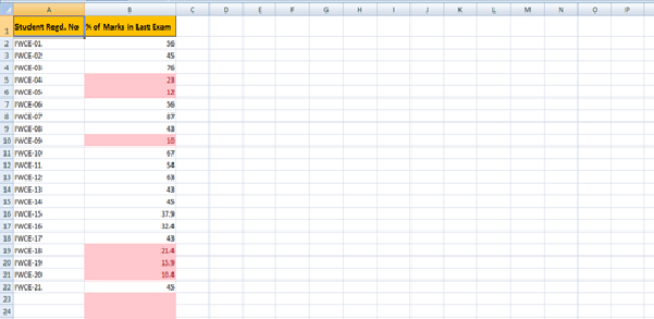
 After you click ok the % of Marks in last exam columns cells marked as red color for which marks smaller than 30.
« Previous
Next »
MICROSOFT EXCEL 2013
CONDITIONAL FORMATTING
MS Excel 2007 Conditional Formatting feature enables you to format a range of values so that values outside certain limits, are automatically formatted. Choose Home Tab >> Style group >> Conditional formatting dropdown Various conditional formatting options:
- Highlight Cells Rules: It opens a continuation menu with various options form defining formatting rules that highlight the cells in the cell selection that contain certain values, text, or dates, or that have values greater or less than a particular value, or that fall within a certain ranges of values.
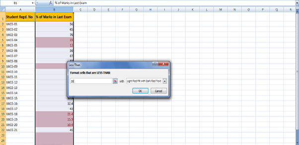
Suppose you want to fund cell with Percentage of marks < 30 and Mark it as red. Choose Range of cell >> Home tab >> Conditional formatting Drop Down>> Highlight Cell Rules >>Less than
After you click ok the % of Marks in last exam columns cells marked as red color for which marks smaller than 30.
- Top/Bottom Rules: It opens a continuation menu with various options for defining formatting rules that highlight the top and bottom values, percentages, and above and below average values in the cell selection.
- Data Bars: It opens a palette with different color data bars that you can apply to the cell selection to indicate their values relative to each other by clicking the data bar thumbnail.
- Color Scales: It opens a palette with different three- and two- colored scales that you can apply to the cell selection to indicate their values relative to each other by clicking the color scale thumbnail.
- Icon Sets: It opens a palette with different sets of icons that you can apply to the cell selection to indicate their values relative to each other by clicking the icon set.
FILL
Fill provides you to fill the content of the cell to up, down, left and right of the neighbouring selected cells. Ex: Suppose you want to fill the content of the cell to down do the follow steps:
- Select the content cell and number of cells to fill down.
- Press Ctrl+D Or Click on Home Tab >>Click on fill from editing group and choose Fill down option.

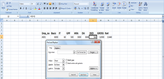
FIND AND REPLACE
Find and select the specified text, formatting or type of information within the worksheet and also can replace text with new text and formatting. To access find and replace dialog box: Click on Home tab >>Find& Select>>Find or Press Ctrl+F
Using Symbols
In some cases you need to insert symbols or special characters which are not available in Keyboard so you can use symbol option from insert tab. To access symbol dialog box:- Click on Insert Tab >>Symbol (from text group) and Symbol dialog box will display.
- Click on a symbol you want.
- Click on insert button.
For Special Character:
- Select the special character tab.
- Click on a special character.
- Click on insert button.